We describe, and show results from, a simple program for simulating the various LHC Computing Models. Currently, the models of particular interest include:
The simulation tool allows us to identify, for each model, probable required bandwidths between the collaborating institutes, limits on the types and number of computing tasks that could be carried out at the collaborating institutes, and order-of-magnitude estimates of the financial cost of the required computing infrastructure.
The simulation technique is very loosely based on work done for SHIFT in the early 90's. Once enough experience has been gained with this simulation, a more sophisticated simulation should be constructed using a commercial WAN modelling tool such as COMNET III. Initial impressions of COMNET III as a tool for this purpose are included at the end of this document.
The simulation program allows for model features that include:
The simulation program calculates the following information:
The following entities are specified as model input:
The collaborating institutes, each institute being characterised by the following data (specified by the modeller):
The computing tasks that may be run at the collaborating institutes, characterised by the following data (specified by the modeller):
The simulation is based on time slices. The clock starts at time T=0.0 and ticks every delta seconds, where delta is chosen to give 10 clock ticks for the smallest data set transfer at the largest available data rate. This ensures sufficiently accurate simulation of small data set transfers.
At each clock tick, the task mix for each collaborating institute is examined. One or more tasks may then be created at the institute, depending on the assigned "probability" of the task when compared with the value of a random number. Example: At FNAL, a "Reconstruction" task of "probability" 100.0 will be started, on average, every 100 seconds. Alternatively, if the task mix assigns a total number to a task, then the required frequency to achieve this number is assigned to the task.
Each created task begins at step 1 of its sequence. A "reconstruction" task might be specified as follows:
      Nsteps = 3
      Step 1 : Get 1.0 MBytes of Raw Data from CERN
      Step 2 : Process for 100 elapsed seconds
      Step 3 : Put 50 kBytes of Reconstructed Data to CERN
whereas a "simulation" task might be specified as:
      Nsteps = 2
      Step 1 : Process for 100 elapsed seconds
      Step 2 : Put 1.0 MBytes of Simulated data to "local" file
At each clock tick, every task is examined to determine whether the current step of the task has completed. If so, then the task is either moved on to its next step, or marked as having terminated.
For tasks where a total number is to be achieved, the assigned frequency for the task is re-computed at each time step accordingly.
The simulation continues running until the time limit (specified by the modeller) is reached, whereupon various statistics are printed out.
For tasks that begin a network transfer step, a "virtual circuit" is established between the institute at which the task is running, and the institute where the data reside. For connections between two different institutes, an Adjustable Bit Rate (ABR) mechanism is assumed for the ATM switch. Each new virtual circuit is thus assigned a data rate for the transfer calculated as the WAN bandwidth model parameter divided by the number of currently active virtual circuits between the two institutes. This calculation is re-done whenever a virtual circuit is created or destroyed on the switch.
For local connections, the virtual circuit is assigned the full ATM rate, and an aggregate rate is calculated and histogrammed for the LAN switch at each time step. The intention here is to allow potentially unlimited backplane or site-wide LAN rates. The histogram of the aggregate rates that actually occured during the simulation gives an indication of the required speed of access to storage implied by the rest of the model.
To obtain a very approximate idea of the financial cost implied by a particular computing model, we specify the following parameters for each institute:
(For dollars read "arbitrary currency unit" in the list above.) Then, at the
end of the simulation, we calculate for each institute (1) the cost of the required
processing power (i.e. the peak number of 100 MIPS processors that was required during the
simulation multiplied by A), (2) the cost of the disk capacity (i.e. the total disk
capacity required to store both data read, and data written, multiplied by B), and (3) the
cost of the WAN links (i.e. the number of WAN links required, multiplied by the ATM rate
as a fraction of 2 Mbits/sec, multiplied by C).
Most of these costs are of course highly speculative. For example, it is not possible today to lease lines running at more than 2 Mbits/sec in Europe. The tariffs for 2 MBits/sec lines runs at around 30000 CHF for one month of lease of a half-circuit to a country neighbouring Switzerland. We thus use a sliding scale that gives a cost of 30000/1.5 = 20000 dollars for a 2 Mbits/sec line, and double that for a 4 Mbits/sec line, and so on...
In the end we sum all the institute costs to arrive at a global model cost figure. The global cost represents the cost of the infrastructure required to perform the given task. The processor part of the cost is invariant under the number of times the given task needs to be performed because, given that the specified processing capacity is installed, then those processors can be used for a continuous series of such tasks. The network costs, on the other hand, go in multiples of a month. If reconstruction continues for 100 days, then three months of lease must be paid, and the network cost must be multiplied by three. The cost of the disk space required for such a run depends on whether the disks are used as a cache or as a permanent store of the data. This area requires further study and modelling.
The prototype simulation program is coded in Fortran 77 and works by first reading in a description file that contains the parameters for the required run.
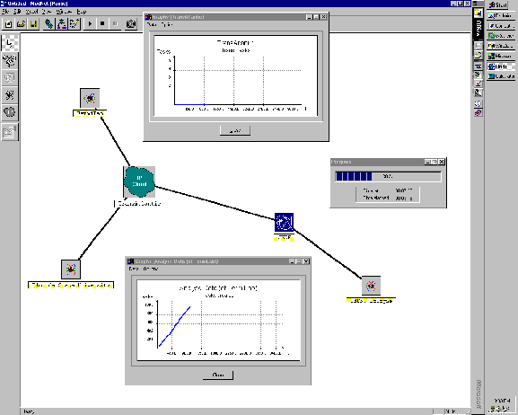
The production tool has been completely re-written in Visual C++ using MFC (Microsoft Foundation Classes), and has a GUI that allows full control over all elements of the model, including real-time graphing of traffic and load. The screen shot below shows the production tool in use.

We show in the following sections results from simulating the various scenarios. These results are also tabulated in an Excel spreadsheet. Note that, since ATM offers only about a 70% payload factor (i.e. the actual data that can be moved across an ATM switch is equivalent to about 70% of the nominal switch rate), the network costs shown in the figures below are underestimated by that amount.
Using the program described, we have simulated the task of a full analysis of a single physics channel in the Central, Regional Centres and Fully Distributed scenarios, under the following assumptions:
Note that the Analysis requires there to already be available 10**7 simulated events: the generation of these events is not modelled.
In the table below, we show the WAN data rates at CERN implied by the task size. For comparison, the average rate seen leaving CERN on WAN lines is currently around 0.5 MBytes/sec (i.e. 40 GBytes per day).
                    Data Moved to Institutes        Aggregate Rate at CERN
                           (GBytes)                      (MBytes/sec)

Central                         0                               0
Regional                      350                             4.0
Distributed                   398                             4.6
We show in the figure below the cost variations in the three cases Central analysis, Regional analysis and Distributed analysis. The infrastructure costs used were:
The WAN costs are calculated using the minimum possible speed required to complete the analysis in the alloted time.
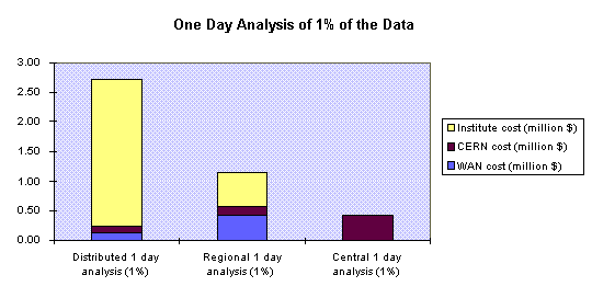
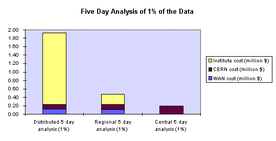
Under the same conditions, we describe an analysis of 1% of the data in a run over 5 days.
We show again the WAN data rates at CERN implied by the task size.
                    Data Moved to Institutes        Aggregate Rate at CERN
                           (GBytes)                      (MBytes/sec)

Central                         0                               0
Regional                      350                             0.8
Distributed                   398                             0.9
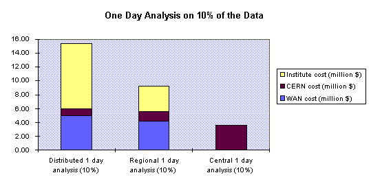
Under the same conditions, we describe an analysis of 10% of the data in a run over a single day.
We show again the WAN data rates at CERN implied by the task size.
                    Data Moved to Institutes        Aggregate Rate at CERN
                           (GBytes)                      (MBytes/sec)

Central                         0                               0
Regional                     3500                            40.0
Distributed                  3980                            46.0
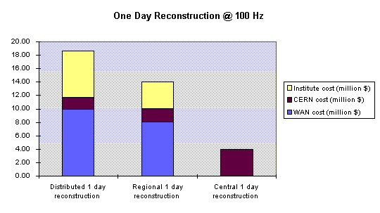
Using the program, we have also simulated the task of synchronous LHC event reconstruction in the Central, Regional Centres, and Fully Distributed scenarios, under the following assumptions:
Here are the WAN data rates at CERN implied by the task size.
                    Data Moved to Institutes        Aggregate Rate at CERN
                           (GBytes)                      (MBytes/sec)

Central                         0                               0
Regional                     7560                            87.5
Distributed                  8597                            99.5
As a learning exercise with the commercial WAN modelling tool COMNET III, we have made a very simple LHC computing model that can be seen in the figure below:

The model is simple in that it simulates only one remote institute. The remote institute is connected to CERN via a WAN ATM cloud via CISCO-type routers at each end. At the remote institute are modelled three different workstation types: one that is running simulation, one that is running analysis, and one that is running reconstruction. Bear in mind that all components of the model as shown can be replicated and grouped as necessary. This means that, once one is satisfied that the components of the simple model are being simulated correctly, then one can scale up the simulation by, for example, having twenty simulation workstations, and fifty remote institutes.
Returning to the model, the tasks that run on the workstations are modelled as step-wise sequencies. The "Reconstruct Event Remote" task, for example, consists of the following atomic steps:
The task itself can be scheduled to run in many different ways. These include the task running every so many seconds, the task running for so many events, the task running randomly according to a user-defined probability function, or the task running on reception of a message. In the model shown I chose the task to run to reconstruct 1000 events i.e. in a loop.
The model, when run, can be animated and real-time graphs can be plotted of, for example, congestion on the CERN FDDI, or I/O rates to the local workstation disks. This is quite good fun to watch. In fact, building a model using this tool is entertaining, but there is a rather steep initial learning curve. The development of various "scenarios" is well supported, allowing the modeller to see the effects of, for example, a network link becoming unavailable, or the effects of an disk I/O bottleneck at CERN.